library(pwr)2 {pwr} basics
In this chapter, the aim is to give tutorial on how functions from pwr (Champely 2020) packages works. This package comes with handful of handy functions to calculate sample sizes and power analysis with some useful plot to visualize sample size and power. The subsequent chapters will shows usage of each functions.
To read the full documentation, you can visit the official {pwr} vignette, which also gives much of the references here.
2.1 Basic Usage
The main function to calculate sample size or power generally in the form of pwr.stats_type.test().
pwr.p.test(): one-sample proportion testpwr.2p.test(): two-sample proportion testpwr.2p2n.test(): two-sample proportion test (unequal sample sizes)pwr.t.test(): two-sample, one-sample and paired t-testspwr.t2n.test(): two-sample t-tests (unequal sample sizes)pwr.anova.test(): one-way balanced ANOVApwr.r.test(): correlation testpwr.chisq.test(): chi-squared test (goodness of fit and association)pwr.f2.test(): test for the general linear model
The basic arguments of these functions are:
Effect size: depending on the specific functions used (e.g.,
his used in one or two-sample proportion test)n: the sample sizes (usually, for each comparison groups)sig.level: A type I error (\(\alpha\)), probability of not rejecting the null hypothesis when it is false, usually default to0.05.power: A power (\(1 – β\)), probability that the test will correctly reject the null hypothesis when the alternative hypothesis is true, usually default to0.08.alternative: “two.sided”, “less”, or “greater”.
From arguments 1 to 4 above, the key idea is to leaves whichever one you want to calculate as NULL (i.e., just don’t fill it).
2.2 Sample size & Power Calculation
For example, given we want to do a one sample t-test, with effect size (d) = 0.5, significant level = 0.05, and power = 0.8.
To calculate sample size, just leaves n and provide the rest:
# Find `n`
pwr.t.test(d = 0.5,
           sig.level = 0.05, power = 0.8,
           type = "one.sample", alternative = "two.sided")
     One-sample t test power calculation

              n = 33.36713
              d = 0.5
      sig.level = 0.05
          power = 0.8
    alternative = two.sided
The sample size (n) = 34
To calculate power (given, say n = 20), just leave power (or set to NULL):
# Find `n`
pwr.t.test(d = 0.5,
           n = 20,
           sig.level = 0.05,
           power = NULL,
           type = "one.sample", alternative = "two.sided")
     One-sample t test power calculation

              n = 20
              d = 0.5
      sig.level = 0.05
          power = 0.5645044
    alternative = two.sided
Power = 0.5645044
2.3 Plotting
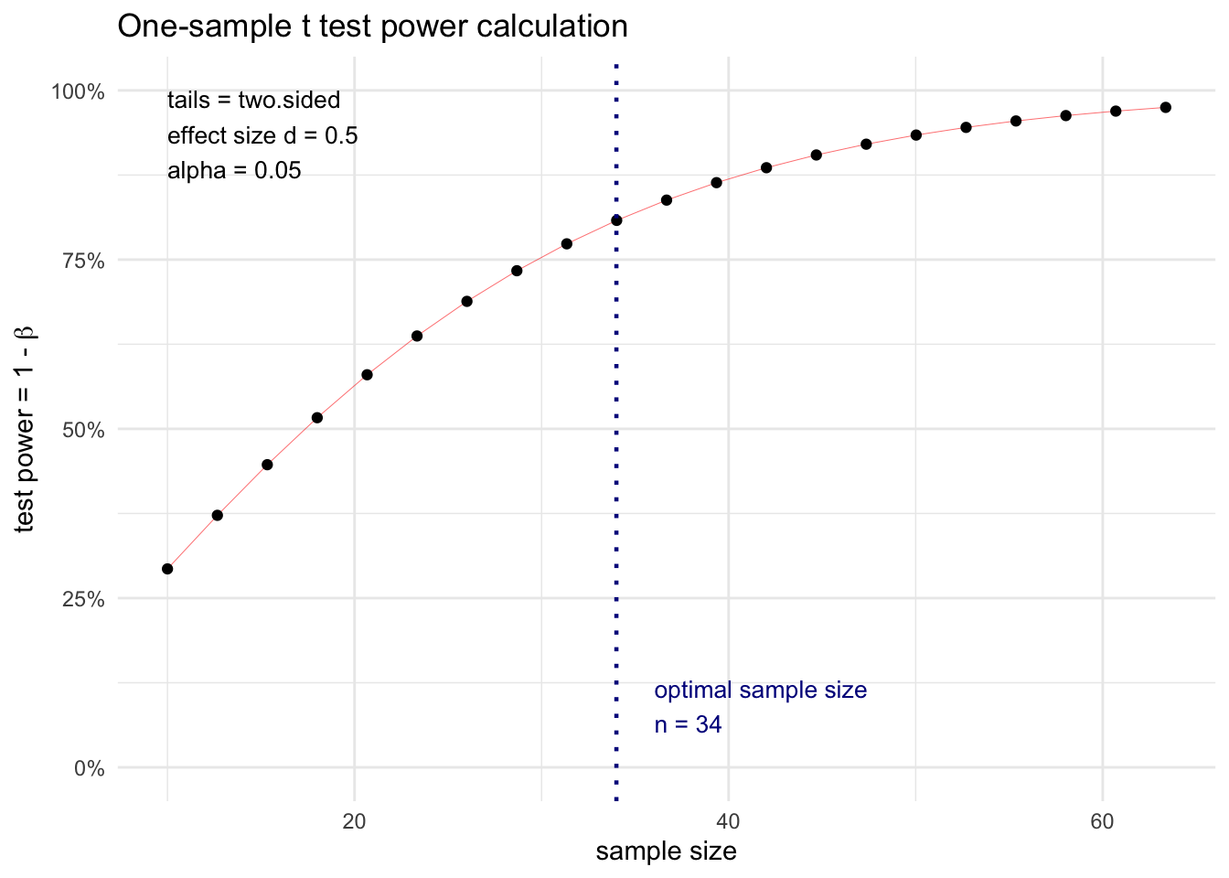
pwr (Champely 2020) provides handy plot() methods to visualized how power changes as sample size changes (and vice versa).
First, assign the result of pwr.*() functions to an object. Then, simply called plot().
res.t.1 <- pwr.t.test(
  d = 0.5,
  sig.level = 0.05, power = 0.8,
  type = "one.sample", alternative = "two.sided"
)

res.t.1
     One-sample t test power calculation

              n = 33.36713
              d = 0.5
      sig.level = 0.05
          power = 0.8
alternative = two.sidedlibrary(ggplot2)
theme_set(theme_minimal())plot(res.t.1)
(It will try using ggplot. if not installed, base R plot will be used.)
2.4 Effect Size
pwr comes with function to compute Conventional Effect Sizes for each type of tests:
| Conventional Effect Sizes | |||
|---|---|---|---|
| small | medium | large | |
| tests for proportions (p) | 0.20 | 0.50 | 0.80 |
| tests for means (t) | 0.20 | 0.50 | 0.80 |
| chi-square tests (chisq) | 0.10 | 0.30 | 0.50 |
| correlation test (r) | 0.10 | 0.30 | 0.50 |
| anova (anov) | 0.10 | 0.25 | 0.40 |
| general linear model (f2) | 0.02 | 0.15 | 0.35 |
cohen.ES() can be used to obtain such effect size for each test.
cohen.ES(test = "t", size = "medium")
     Conventional effect size from Cohen (1982)

           test = t
           size = medium
    effect.size = 0.5
Or as a shortcut, passing string describing the strength directly to pwr*().
pwr.t.test(d = "medium",
           sig.level = 0.05, power = 0.8,
           type = "one.sample", alternative = "two.sided")
     One-sample t test power calculation

              n = 33.36713
              d = 0.5
      sig.level = 0.05
          power = 0.8
    alternative = two.sided
2.5 Internals
2.5.1 Sample size & Power
The object from pwr.*() functions stores information of each arguments you’ve called and its calculation.
sloop::otype(res.t.1) # Object Type[1] "S3"class(res.t.1) # Special class[1] "power.htest"str(res.t.1)List of 7
$ n : num 33.4
$ d : num 0.5
$ sig.level : num 0.05
$ power : num 0.8
$ alternative: chr "two.sided"
$ note : NULL
$ method : chr "One-sample t test power calculation"
- attr(*, "class")= chr "power.htest"# To get individual arguments for further calculation
res.t.1$n[1] 33.36713res.t.1$power[1] 0.82.5.2 Effect size
Effect size can also be obtained from cohen.ES()
es.t.med <- cohen.ES(test = "t", size = "medium")
class(es.t.med)
[1] "power.htest"str(es.t.med)List of 4
$ test : chr "t"
$ size : chr "medium"
$ effect.size: num 0.5
$ method : chr "Conventional effect size from Cohen (1982)"
- attr(*, "class")= chr "power.htest"es.t.med$effect.size[1] 0.5